
This week I am going to show you some very basic things you can do with GPS coordinates. In this post you will learn how to:
- Read gpx files
- Read files containing plain text coordinates (like N 48 12.123 and N 48 12′ 123″)
- Parse characters string that contain unformatted coordinates (like above)
- Convert minute and second format to decimal format for easier processing
- Compute distances, angles and antipodes using the package geosphere
- Create a basic plot of a gps track
Contents
Read gpx files
Ok, so reading them is easy, you just need an XML library. But if you want to use them for further processing it is probably best if you convert it into a data.frame. This can be done with the following method:
readTrackingFile<-function(filename) {
  require(XML)
  require(plyr)
  xmlfile<-xmlParse(filename)
  xmltop<-xmlRoot(xmlfile)
  tracking<-ldply(xmlToList(xmltop[['trk']][['trkseg']]), function(x) {
    data.frame(x)
  })

  tracking<-data.frame("ele"=tracking$ele[seq(1, nrow(tracking), 2)], "time"=as.character(tracking$time[seq(1, nrow(tracking), 2)]),"lat"=tracking$.attrs[seq(1, nrow(tracking), 2)], "lon"=tracking$.attrs[seq(2, nrow(tracking), 2)])

  tracking$ele<-as.numeric(levels(tracking$ele))[tracking$ele]
  tracking$lat<-as.numeric(levels(tracking$lat))[tracking$lat]
  tracking$lon<-as.numeric(levels(tracking$lon))[tracking$lon]

  x<-strptime(as.character(tracking$time), "%Y-%m-%dT%H:%M:%SZ")
  tracking$min<-60*x$hour + x$min

  message(paste("read", nrow(tracking), "tracking points"))

  return(tracking)
}

track<-readTrackingFile("data/LJWSIZUT_04_11.gpx")
head(track)
First we read the file using an XML library, then we get the root element and then use ldply (which is pretty cool!) to transform the whole thing into a data.frame. Just like that. I have to admit I did not come up with this on my own, but I do not remember where I got it from, probably stackoverflow. 'trk' and 'trkseg' are XML-elements as you probably figured out.
But so far you only get a data.frame which has a separate row for lon and lat values, that is because they are attributes. Below you see the structure of the gpx file:
Generated by Tractive Platform Service
Tracker LJWSIZUT, 2015-04-12T09:59:34+00:00 2015-04-11T22:14:13Z
419
[...]
And here you can see the first two rows of the data.frame after ldply:
     .id ele                 time     .attrs
1  trkpt 419 2015-11-04T13:12:32Z 48.3201233
2  trkpt 419 2015-11-04T13:12:32Z 14.6258633
That is why I applied
tracking<-data.frame("ele"=tracking$ele[seq(1, nrow(tracking), 2)], "time"=as.character(tracking$time[seq(1, nrow(tracking), 2)]),"lat"=tracking$.attrs[seq(1, nrow(tracking), 2)], "lon"=tracking$.attrs[seq(2, nrow(tracking), 2)])
which selects every other row for elevation and time, but each row for latitude and longitude.
Afterwards the method only converts the factors to numerics (more on factors) and convert the time into minutes from midnight (I will be using this data for a project and the time might be useful).
The input file I use is a tracking file from my Tractive GPS Pet Tracking device. You can download it here.
The output of the above code looks like:
  ele                 time      lat      lon min
1 419 2015-11-04T13:12:32Z 48.32012 14.62586 792
2 399 2015-11-04T13:48:51Z 48.32021 14.62588 828
3 384 2015-11-04T13:54:23Z 48.32028 14.62590 834
4 391 2015-11-04T14:58:33Z 48.32027 14.62588 898
5 422 2015-11-04T15:08:33Z 48.32006 14.62588 908
6 439 2015-11-04T15:19:01Z 48.32008 14.62632 919
Read plain text coordinates
Sometimes you might encounter coordinates like this:
48° 22.124'
48° 22.134
48°22.123
48°22.123'
48 22 123
48° 22' 123"
48°22'123"
First I thought this could not be a problem but R taught me otherwise. The solution that works for me is the following:
testLines<-read.table("testCoords.txt", sep=";", header=F, quote="", stringsAsFactors = FALSE)$V1
testLines
which prints:
[1] "48 22.123" "48° 22.124'" "48° 22.134" "48°22.123" "48°22.123'" "48 22 123" "48° 22' 123\"" "48°22'123\""
- Why not use readLines()? The problem with readLines(), at least for me, was that it encountered and "incomplete final line found on testCoords.txt" when there is not an extra empty line after the last coordinates.
- sep=";": This can be any separator except a space.
- quote="": Otherwise you get problems with the second symbol ("). (stackoverflow)
The most important thing for me was to set the locale settings, because before that R always replaced the degree symbol by some ASCII representation ...
Sys.setlocale("LC_ALL", 'en_GB.UTF-8')
Otherwise not even changing the encoding of the file and using the encoding parameter worked for me!
Parse character strings
So, now we have read these unformatted gps coordinates, but we can not compute anything with them. So I wrote a parsing function, that should cover the cases that I could think of.
parseCoord<-function(coordChar) {
  if (!is.character(coordChar)) {
    stop("coord is not in character format.")
  }
  coordChar<-trim(coordChar)
  direction<-substr(coordChar, 1, 1)

  if ((direction %in% c("N", "E", "S", "W"))) {
    coordChar<-substr(coordChar, 2, nchar(coordChar))
    coordChar<-trim(coordChar)
  }

  splitted<-unlist(strsplit(coordChar, "[ °'\"]"))
  splitted<-splitted[which(splitted!="")]
  deg<-as.numeric(splitted[1])

  min<-NULL
  sec<-NULL

  if (length(splitted) > 1) { # means it also contains minutes
    min<-as.numeric(splitted[2])

    if (length(splitted) > 2) { # means it also contains seconds
      sec<-as.numeric(splitted[3])
    }
  } else {
    warning ("your coordinates do not seem to contain minutes.")
  }

  return(list("dir"=direction, "deg"=deg, "min"=min, "sec"=sec))
}
This function works for formats that contain °, " and ' as symbols, but also without them. And it does not matter whether there is an additional space before/after each symbol. Giving a direction (N, S, E, W) is also optional.
Check and convert coordinates
So far we have read and parsed different coordinate formats, but we still can not compute with them. So I wrote methods to convert my rather simple coordinate format to a decimal format.
We need a little helper function which I found on stackoverflow.
trim <- function (x) gsub("^\\s+|\\s+$", "", x)
First I created two methods two check the format, so that the user can not just put anything into the conversion methods:
isSecond<-function(coord) {
  if (is.null(coord[["deg"]])) { return (FALSE) }
  if (is.null(coord[["min"]])) { return (FALSE) }
  if (is.null(coord[["sec"]])) { return (FALSE) }

  if (!is.numeric(coord[["deg"]])) {return (FALSE) }
  if (!is.numeric(coord[["min"]]) || coord[["min"]] > 60 || coord[["min"]] < 0) {return (FALSE) }
  if (!is.numeric(coord[["sec"]]) || coord[["sec"]] > 60 || coord[["sec"]] < 0) { return (FALSE) }

  return (TRUE)
}

isMinute<-function(coord) {
  if (is.null(coord[["deg"]])) { return (FALSE) }
  if (is.null(coord[["min"]])) { return (FALSE) }
  if (!is.null(coord[["sec"]])) { return (FALSE) }

  if (!is.numeric(coord[["deg"]])) { return (FALSE) }
  if (!is.numeric(coord[["min"]]) || coord[["min"]] > 60 || coord[["min"]] < 0) {
    return (FALSE)
  }
  return (TRUE)
}
The conversion functions are a lot shorter and pretty simple:
min2dec<-function(coord) {

  if (!isMinute(coord)) {
    stop("coord is not in minute format.")
  }
  dec <- coord$deg + coord$min / 60
  return (dec)
}

sec2dec<-function(coord) {
  if (!isSecond(coord)) {
    stop("coord is not in second format.")
  }
  dec <- coord$deg + coord$min / 60 + coord$sec / 3600
  return (dec)
}
Compute distances, angles and antipodes
Now we can finally compute things.
There are basically two ways how to compute distances on earth ("Great circle" and "Rhumb line"), but this would be enough information for another post. For now we are going to focus on "Great circle" or "as the crow flies" (german: Fluglinie).
The package geosphere introduces three different methods for computing distances along the "great circle". As an example we compute the distance between my cat (the first tracking point) and our house.
distMeeus(c(track$lon[1], track$lat[1]), c(house$lon, house$lat))
The result is:
[1] 12.91136
distCosine(c(track$lon[1], track$lat[1]), c(house$lon, house$lat))
The result is:
[1] 12.92392
distHaversine(c(track$lon[1], track$lat[1]), c(house$lon, house$lat))
The result is:
[1] 12.92394
The results are in meters and we can see that there are already some differences. This is because the methods distCosine() and distHavarsine() assume a spherical earth and distMeeus() assumes an ellipsoid earth which is a lot more accurate.
To see a bigger distance I computed the distance between the northpole and my house (in km):
northpol<-list("lat"=90, "lon"=0)
distMeeus(c(northpol$lon, northpol$lat), c(house$lon, house$lat))/1000
The result is:
4647.923
distCosine(c(northpol$lon, northpol$lat), c(house$lon, house$lat))/1000
The result is:
4639.77
distHaversine(c(northpol$lon, northpol$lat), c(house$lon, house$lat))/1000
4639.77
Interestingly, the first method now computes a longer distance than the two other methods (in contrast to the cat-house example) and the two spherical methods even have the same result.
So, now I know how far I am away from the northpole and more important, from my cat. The next thing I need to find out is in what direction I have to walk to get to her:
bearing(c(house$lon, house$lat), c(track$lon[1], track$lat[1]))
The result is:
168.3352
Here it is important to use the starting point as the first parameter!
What can also easily be computed with the geosphere package is the antipode of a point.
antipode(c(house$lon, house$lat))
The result is:
-165.3742 -48.32024
You might figure out that you simply have to switch the sign for the latitude and you have to distract 180 for the longitude 🙂
Create a basic plot of a gps track
Finally my favourite part, plotting!
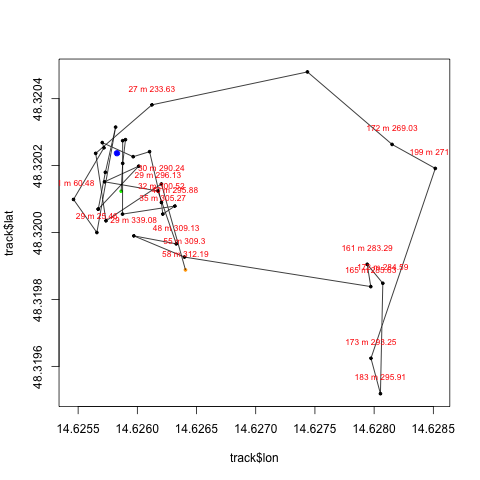
First, lets create a plot of my cats tracking points (marking the first one green and the last one orange):
plot(track$lon, track$lat, pch=19, cex=0.5, col=c("green", rep("black", length(track$lon)-2), "orange"))
Add the position of my house, to see roughly where my cat likes to go:
points(house$lon, house$lat, col="blue", pch=19)
Add lines to connect the dots:
lines(track$lon, track$lat)
The next thing is just a little playing around, I added the distance and the bearing to each datapoint:
for (i in 1:length(track$lon)) {
  d<-round(distMeeus(c(track$lon[i], track$lat[i]), c(house$lon, house$lat)), digits=0)
  if (d > 25) {
    a<-round(bearing(c(track$lon[i], track$lat[i]), c(house$lon, house$lat)), digits=2)
    text(track$lon[i], track$lat[i] + 0.00005 , labels=paste(d, "m", a), col="red", cex=0.7)
  }
}
And that is the final plot:
And here you can download the complete source used in this tutorial.