In my job and my studies I recently finished I work with lots of different data sources and you will also meet all of them throughout your career as a data scientist. Data can be given to you as an SQL dump, XML files and many other formats. In my experience most often data is handled in Excel or .csv (comma separated values) files. Therefore Microsoft Excel is very useful to get a first impression of the data and to prepare them for further data processing.

In this post I’ll show how a data set, that’s available as a table, can be displayed, filtered and analysed with the help of the table tools in Excel.

Data

For this post I downloaded a dataset from the Machine Learning Repository: Go to the download page of the Online Retail dataset

The following columns are contained:

• InvoiceNo
• StockCode
• Description (Product Name)
• Quantity
• InvoiceData
• UnitPrice
• CustomerID
• Country

Read data

If a dataset is not available as an Excel file but as a .csv (comma separated values) or .tsv (tab separated file) and you want to open it with Microsoft Excel, you can use the Text Import Wizard. This function and several other (e.g. import from HTML or a database) can be found at the tab View. Under the following link you can find a manual about Import or export from text files. If the separating character is compatible with the language of your Excel version a file can simply be opened with a right click > Open with > Excel …

The first 2 steps that I usually do in the beginning of working with a file are:

• Freeze panes
• Activate the filter function

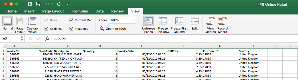
Freezing panes works like this: Highlight the first row, go to View and click on Freeze panes. If the second row should also be frozen, mark the third row and click Freeze panes again. The same applies to any further row you want to freeze. This function results in having the first row fixed and after that you can always see the column names when you scroll down in a large document.

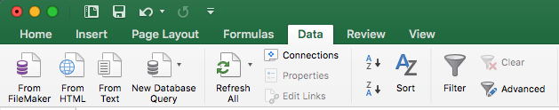
In the tab Data you can find the function Filter. If you activate it next to each column name a small arrow appears. Clicking on it makes it possible to filter or sort the table by this column. This is also useful to see which values can appear in this column.

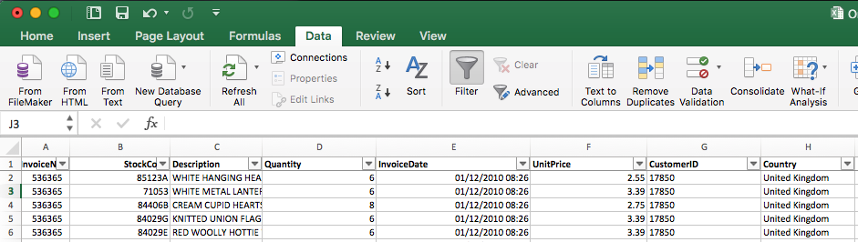
Table functions

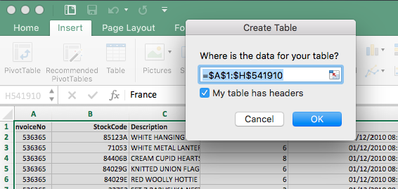
If you plan to work with your file longer than a few minutes, it might make sense to insert a table altogether instead of using just the filter functions. A table provides the user with several useful functions. To insert it you need to mark the area that holds the data and convert it to a table by clicking Insert > Table.

A table has several advantages:

• Filtering & sorting like shown above
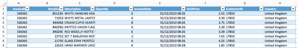
• Formatting: You get a better overview because of banded rows
• Several function in Table Tools (explained below)

Use formulae

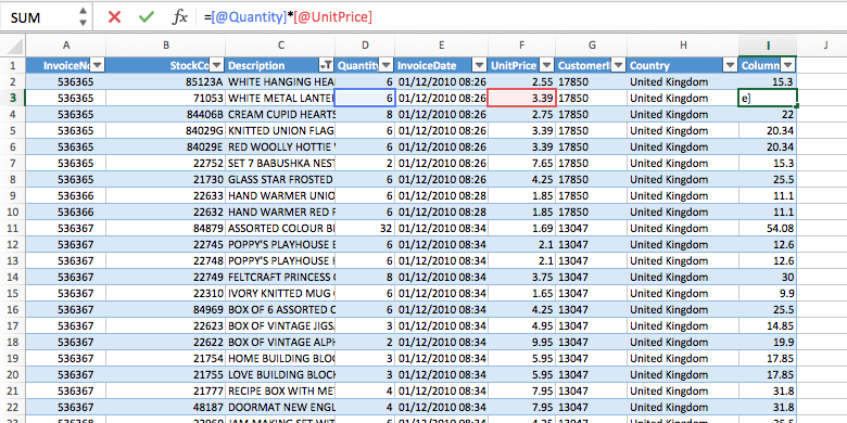
With Excel I usually associate the many different formulae that you can use on cells, columns and rows. In this context the drag function is very useful because you can copy formulae to adjacent cells while automatically updating the variables. In my dataset it might be interesting to multiply Quantity and UnitPrice to compute the total price. Without using a table, we would need to type =D2*F2 into the next free column, click at the fill handle and drag the cell down until the last row of the table. Since we have more than 500.000 cells this might take a while.

When you are using a table, this is a lot easier. You simply click in the first free column and type =[@Quantity]*[@UnitPrice] (or click the columns instead of typing their names). The first advantage that is immediately visible is that you can use column names for referencing and the second benefit is that you don’t need to drag the formula to all other cells anymore. After you enter the formula the complete column is immediately filled with the computed values and also inherits the formatting.

Table tools

When you click into any cell inside the table a new tab called Table appears.

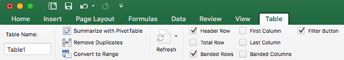
Here you have many possibilities:

• Summarize with PivotTable: This function will be explained further below.
• Remove Duplicates
• Convert to Range
• Switch Header Row on/off: The Header Row is switched on by default and I don’t see any reason why it should be switched off as long as there are useful column names. When you scroll down and the first row is not visible anymore, instead of the column names A, B, C, … the names of the first row appear.
• Total Row: This function will be explained further below.
• Banded Rows: Paints the rows alternately in two different colours for better overview.
• First / Last Column: Print the values in the first / last column bold face.
• Filter Button: With this you can activate / deactivate the small filter arrow next to each column name.

Prepare data for further processing

Before I apply Total Row and the function Summarize with PivotTable, I’ll filter out some useless product names that I noticed when scrolling over the data. For this click on the small arrow next to the column “Description” and remove the tick from every value that you don’t need. I removed the first value because it’s a number, every value that starts with a ? (I guess that are erroneous values) and the last value “(BLANK)”, because those are empty rows.

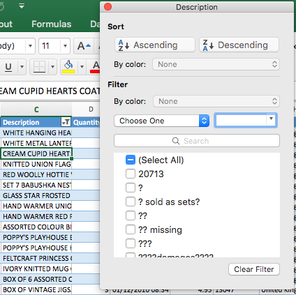
Next to the arrow a funnel appears so that you can see whether a column was filtered.

Total row

Since it’s a very useful function I want to introduce Total Row. To activate it you need to check the box next to “Total Row” in the ribbon.

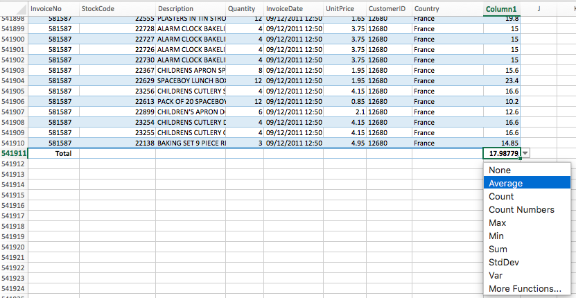
At the bottom of the table you will now see a new row. In each of the new cells is a list of functions that can be applied to the columns, but not every function is useful for every type of data. For our new column that contains the total price, we could compute the average or the sum.

PivotTable

One really interesting thing are pivot tables. Pivot has the same or similar meaning as rotate and that is a useful meaning for this operation because we can actually “rotate” the content of a column to become the content of a row. In this table we would like to find out how many items we have sold of each product. Because the table is so big it doesn’t make sense to sort it and then try to manually count the sold items. For this purpose we can use a PivotTable. You have to be in the table (just click inside a cell) and click Summarize with PivotTable.

In the window the table that we just created is automatically selected.

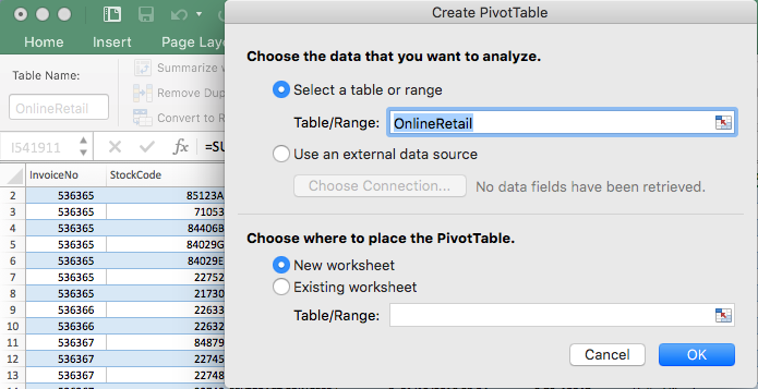
After clicking “OK” the following window appears. There you can select from which column the values for the new column names are picked, which values are used for filtering and which values will make up the content of the new table.

I created the table as follows:

• Filters: You should be able to select by Country or CustomerID
• Columns: The column names should be the values from the column Description
• Rows: For this task we don’t need row names
• Values: The values should be the sum of bought items per product

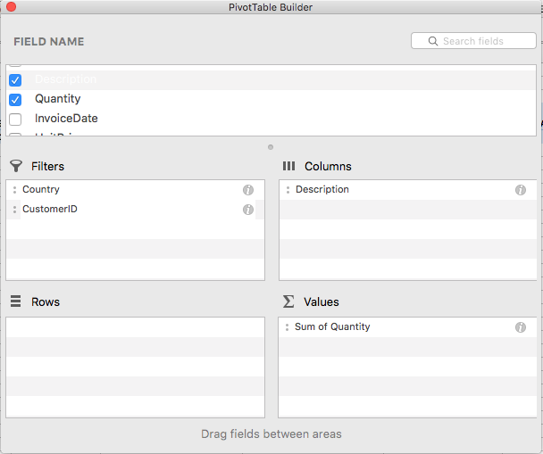
While you are dragging the column names to the desired area, you can already see how the table builds up. As soon as you click on the red circle to close the builder, the PivotTable is finished.

Filtering like I showed above unfortunately is not adopted but by clicking at on the small arrow next to Column Labels the already known filtering dialog appears and you can simply unselect the same values as we did before.

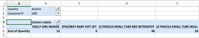
Since I added Country and CustomerID to the filters, we can use the first to find out how many items of each product were sold in Austria. Click on the arrow next to Country and a new dialog appears. Click “(Select All)” to unselect all and then tick the checkbox next to “Austria”. By closing the dialog the filter is applied.

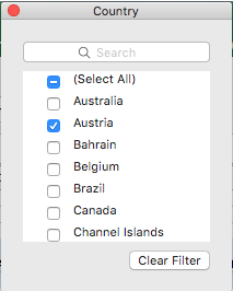
Finally you have a table that displays which products were sold how often to Austria.

Conclusion

Excel has very mighty Table Tools and you don’t always need knowledge about a programming language to get simple statistics out of big tables. The ribbon menus make the program very nice to use and the graphical user interface has improved a lot compared to previous versions.

If you have any questions or suggestions, feel free to leave a comment!