I remember when I had an R course at university I was really not a fan of rmarkdown and knitr. But since I participate in a Learning Club, where people are encouraged to document and present their code, data and results, I started to love it. Prior to that I’ve always documented my assignments at the university either using LaTeX or simply in a Word Document. This required copying and pasting code and even worse, saving each image (or taking a screenshot) and include it into the document. Every time I had to fix something in the code or in the plot, I had to redo that part and everything that was based on it. After I watched Becoming a Data Scientist Podcast: Episode 01 – Will Kurt where Will highly recommends rmarkdown I thought I’d give it another try.
Many users in the Learning Club also mentioned jupyter which is “a web application that allows you to create and share documents that contain live code, equations, visualizations and explanatory text”. It’s written in Python but aims at Python, R and Julia as far as I know and for my purposes I just needed to install the IRKernel additionally.
To find out which tool I’d like best I did the latest activities in the Learning Club and documented one exercise in jupyter and one in rmarkdown.
And since it also doesn’t make sense to repeat what I have said about the three techniques in the corresponding reports, I decided not to write a separate blog post about each, but to focus on how I created the documentation.
Here you can find the activity descriptions:
- Activity 05: Naive Bayes
- Activity 06: k-means Clustering
- Activity 07: Simple Linear Regression
Contents
rmarkdown report for Activity 05: Naive Bayes
As always, the code for this activity can be found in my github repo ds-learning-club/05-naivebayes.
This was the first time that I used rmarkdown without having to use it for university. It’s very similar to markdown which is e.g. use for writing documents and README files in github projects. The first thing that you need to learn are the different settings you can use on code junks because this will make your life a lot easier. You really don’t want time-consuming computations to run everytime that you knit your document into a PDF or HTML file.
- include: should this code chunk be shown in the report?
- eval: should the code in this chunk be executed? Set to
FALSEfor time consuming computations. - echo: should the result of this code chunk also be put in the report?
- cache: should this code chunk be cached? Small changes in the code (even just spaces) will lead to the removal of the cache.
In the following you can see a sample for each of the settings:
{r setup, include=FALSE}
knitr::opts_chunk$set(echo = TRUE)
knitr::opts_chunk$set(cache = TRUE)
include=FALSE is set because I don’t want my settings to show up in the PDF report.
cache=TRUE is set by default because the report has many plots and I don’t want that they are generated everytime I knit the report.
echo=TRUE is set for the whole document because most of the time I want the output to be printed (actually I think it’s the default anyway).
{r knitr, echo=FALSE}
library(knitr)
echo=FALSE is set for this chunk because the library knitr is not related to the topic of this report but required to print nice tables with kable().
{r mushroom, eval=FALSE}
mush_data <- read.csv("https://archive.ics.uci.edu/ml/machine-learning-databases/mushroom/agaricus-lepiota.data", sep=",", header=FALSE)
set.seed(5678)
mush_test <- sample(1:nrow(mush_data), nrow(mush_data)*0.1)
mush_data_melt <- melt(mush_data, id.vars = "edible")
eval=FALSE is set here because reading data takes some time and should therefore be done only once. If I execute the code once in RStudio it's in the workspace. And if I use the "correct" way to knit the document
Here you find everything about knitr options.
At least not always. I was a little bit annoyed that when I finished my analyses and wanted to create a report, all my variables seem to have disappeared and I needed to read all the data again. This is because clicking the "Knit PDF" button creates a new workspace and ignores what is in your current workspace. Before I knew how to properly circumvent this, I did my analyses, saved the outputs as .RData file and loaded the workspace at the beginning of my report. But there is a better solution to this problem:
library(knitr)
knit2pdf("subfolder/my-report.Rmd")
Would be cool if this was a button in RStudio but at least there is a workaround.
Jupyter report for Activity 06: k-means Clustering
The Jupyter notebook for this exercise can be found in my github repo ds-learning-club/06-kmeans.
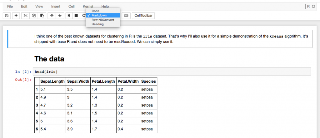
Some people in the Learning Club have been talking about using Jupyter. I was interested in trying it and set it up on my computer. Jupyter is running as a web application and you can open your notebooks in your browser. Like in rmarkdown the pieces you add (here they are called "cells") can have different types.
- Code
- Markdown
- Raw NBConvert
- Heading
But apart from that, rmarkdown and Jupyter are very different. rmarkdown is actually just a markdown language and the reason why it is so great to use for both documentation and interactive analysis is mainly because of RStudio. Jupyter definitely has features that are not available when working with rmarkdown.
- Support of many different languages
- Documents contain live code
- You can save & checkpoint and revert to checkpoints from the menu
It's absolutely an interesting idea and probably useful for many things but when it comes to documenting R code, it's not my first choice. Opiate for the masses has a blog post on why he doesn't like Jupyther which summarises some of the issues I have/had with the Jupyter notebooks.
- Code can only be run in chunks.
- It’s difficult to keep track.
These two things mean that 1) if there are several lines of code in one chunk, you can only run them together and 2) if you are playing around in your notebook, the code chunks might not have been executed in the way that they are displayed, but: at least there is an execution number indicating the order which is a clear advantage over R. Because also in R you can manually execute the code chunks and by changing the settings of the code chunk suppress execution when the report is generated (which makes sense for time consuming computations). And in R you would need to check the history to see the order of the execution.
One thing is also that if you're used to RStudio, you'll be missing the great user interface. Due to how Jupyter is designed, you just have a stream of your commands with their output and some text in between. If you run commands e.g. calling the help for commands, that you'd run in the console of RStudio and not inside your report, it's also there. And if you don't want it anymore you have to delete it. In RStudio the help result would just appear in its own pane.

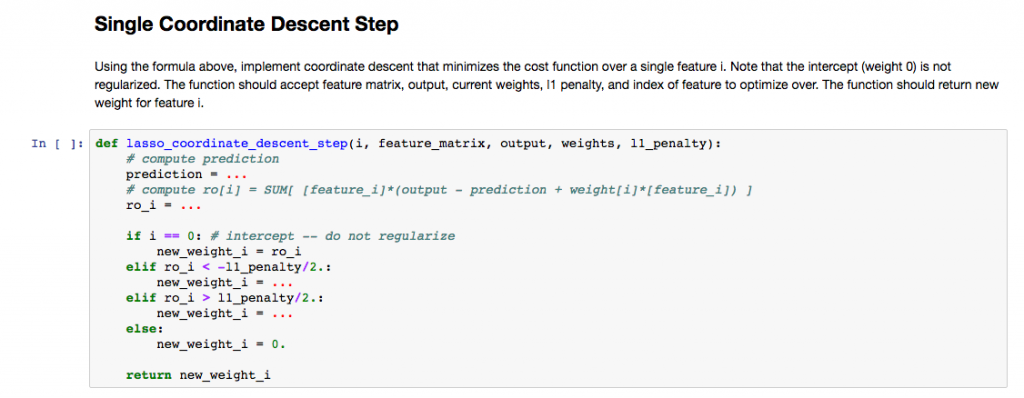
A very practical application for Jupyter is creating exercise sheets like for the Machine Learning course I am currently doing on Coursera. For such a course the lecturer provides a Juptyer notebook with descriptions for the tasks, basic frames for the required functions, test code (to check you functions) and sample code. The course I am currently taking is in Python but of course this can also be done for R courses.
My conclusion is that Jupyter is useful for many things, e.g. if you want to define a workflow, run it from the command line and save the report afterwards. For describing a specific problem I solved or documenting a method or package, rmarkdown will stay my weapon of choice.
rmarkdown report for Activity 07: Simple Linear Regression
This is an exercise I especially enjoyed because I like the topic Linear Regression and always wanted to know more about the package lm().
The code and report for this exercise can be found in my github repo ds-learning-club/07-linear-regression.
Although at that point I had done a few rmarkdown reports (it was a few weeks after I created the Naive Bayes report) while writing this report I really started to appreciate how easy it was to create such a lengthy report (22 pages) without much extra effort.
Code-first vs. Documentation-first
During writing my first documents with rmarkdown, I followed two different approaches. I will explain both of them and suggest when each of them is useful.
- Code-first: I followed this approach with the first report (Activity 05: Naive Bayes). At first I created an R script and did my analyses. After I finished I copied all the bits that I wanted to be in my documentation to an .Rmd file and created the documentation around it. While coding I already noted some things in the comments that I wanted to have in the documentation.
- Documentation-first: For the second report (Activity 07: Simple Linear Regression) I started directly with an .Rmd file. This is especially useful if you have a list of things you want to document (like I did with all methods that can be used on an lm() model. If you do this you can create an outline/structure of your document and start filling your report with code and plots.
For creating the documentation of a certain workflow or a package (like a vignette) I'd chose the documentation-first approach. If I do analysis on a new dataset where most of the time you don't exactly know where it will take you, I'd do code-first (but write down lots of comments). For bigger projects you have to split up your analysis anyway and a mixture of both might be useful
A not so successful undertaking: Post from RStudio to wordpress
Some time ago I found a package called RWordPress but unfortunately the website is down. I contacted the author and he sent me the package. To make sure it doesn't disappear too I forked it to my github account. I started doing some analysis on my own blog posts (nowhere public yet) and thought that it might actually be cool to post blog articles directly from RStudio. Of course I was not the first person to do this and so I found many resources on this:
- How to update your WordPress.com blog from R
- Write Posts With Rstudio, Rmarkdown Format And Publish Directly To WordPress With Knitr & Rwordpress
- Publish blog posts from R + knitr to WordPress
- Using knitr and RWordPress to publish results directly from R
- Rchievement of the day #3: Bloggin’ from R
Using all those links I managed to create a new post on WordPress that contained somehow the content I wanted to have. I was even possible to include my images by using some magic of the knitr package:
opts_knit$set(upload.fun = function(file) imgur_upload(file, key="d56260245fa1e90"), base.url = NULL) # upload all images to imgur.com

opts_chunk$set(fig.width=5, fig.height=5, cache=TRUE)
Unfortunately so far I was not able to format the code in a way that I liked it. It might be some problem with my code formatting plugins, some wrong knitr setting or something else. I tried to manually replace the code and pre tags created by knitr by pre lang="RSPLUS" tags which would be the correct tag for my WP CodeBox plugin to format it correctly.
With my manual formatting I somehow broke the HTML and currently I can't figure out why (number of opening and closing tags is the same and also the Developer Console doesn't show anything). So for now I gave up and decided to write my posts old school, because that experiment took way too much time already.
For writing tutorials and so on it would be really useful but I'll need to give it another shot and maybe try it with a shorter rmarkdown at first before succeeding with this task.
Useful links & tips
Most of these things I found out by searching Google, which most of the time leads to yihui's website.
Other resources I found useful are:
- Working directory is forced for each chunk? If your .Rmd file is not located in your working directory but maybe in a subdirectory, relative paths will not work as you might expect. By setting knitr::opts_knit$set(root.dir = "/Volumes/Vero/Repos/ds-learning-club") (replace it with your working directory) you can use paths relative to your working directory.
- Error line numbers are wrong: This was also a bit annoying. When you use the "Knit PDF" button in RStudio and an error occurs, the error line number is the first line in the erroneous chunk and not the exact line number. When you use rmarkdown::render('test.Rmd') to knit your file, you'll get better debug output.
- Is there a way to knitr markdown straight out of your workspace using RStudio?
I hope this post gave a short introduction to rmarkdown from a practical point of view and showed you why in my opinion it is better suited for documenting R code and projects compared to Jupyter.