
I am planning to write about parametric and non-parametric testing but since I know that many people have difficulties with the concept of hypothesis testing itself, I am going to give an introduction to the basic concepts first without immediately trying to frighten you.
In general, a statistical test consists of four steps:
- Formulate the null hypothesis \(H_0\) and the alternative (or research) hypothesis \(H_1\).
- Identify a test statistic.
- Compute a p-value.
- Compare to an appropriate \(\alpha\)-value. If \(p\leq\alpha\), \(H_0\) can be rejected.
Below follows an exact description of each of these steps. The statistical tests that I am going to publish over the next few posts will all be structured in these four steps to make it easier for you to follow.
Contents
1. Formulate the null hypothesis \(H_0\)
Typical cases for statistical tests are to find out whether:
- a medication works.
- shopping behaviour is different between two groups.
- a disease is more common among a group than among another.
- a variable follows a supposed distribution.
- your method is better than another.
- …
In short: You want to find whether there is a difference between two or more samples. Most of the time people rather see a difference, so it is important to be cautious with published results. The wrong test or even the wrong interpretation of the correct test can lead to the result that the scientist/author expects when in fact there is no significant difference.
\(H_0\), the null hypothesis, is the case that the observed value / observed distribution equals the reference value / reference distribution, e.g.:
$$H_0: \mu_0 = \mu$$
\(H_1\), the alternative or research hypothesis is the case that they are not equal, which can mean the following:
- \(H_1: \mu_0 \ne \mu\) (two-sided test)
- \(H_1: \mu_0 < \mu\) (one-sided test)
- \(H_1: \mu_0 > \mu\) (one-sided test)
So, depending on what you want to test, these are the basic rules for defining the null hypothesis.
2. Identify a test statistic
A test statistic is a measure that describes your sample in one value. How to compute this test value strongly depends on your data, whether you have one or more samples (to compare to a reference value or to each other) and which distribution you assume.
In general you get a test statistic \(t\) from which a p-value can be computed.
3. Compute a p-value
How to compute a p-value depends on the distribution of the test statistic which does not necessarily have to be the same distribution as your sample.
The most used distributions (at least for the statistical tests that are taught in university) are:
- Normal distribution
- Students t distribution
- \(\chi^2\) distribution
- F distribution
The first figure shows the normal distribution and the Student’s t distribution (with different degrees of freedom) side by side.
The normal distribution is defined as:
$$P(x) = \frac{1}{\sigma \sqrt{2 \pi}} \times \exp{\frac{-(x-\mu)^2}{2 \sigma^2}}$$
where \(\mu\) is the mean and \(\sigma^2\) the variance. The standard normal distribution (or z-distribution) has \(\mu=0\) and \(\sigma^2=1\).
This distribution describes full populations (which is important when choosing the reference distribution).
The Student’s t distribution is described by wolfram alpha as “the distribution of the random variable t which is (very loosely) the “best” that we can do not knowing \(\sigma\)”. It describes, in contrast to the normal distribution, samples drawn from a full population.
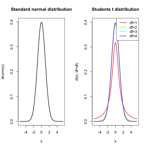
In the plots above we see that the normal distribution and the Student’s t distribution look very similar, more so, when considering higher degrees of freedom. If you do not know yet what degrees of freedom are, don’t worry. You will learn for each statistical test how to compute them. In case of the Student’s t distribution it is the number of samples minus 1.
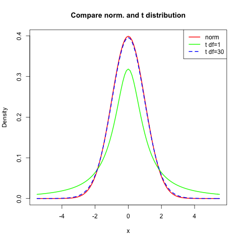
Because the densities look so similar I compared the normal distribution to two different t distributions. You can see that the t distribution with 30 degrees of freedom pretty much is like the normal distribution.
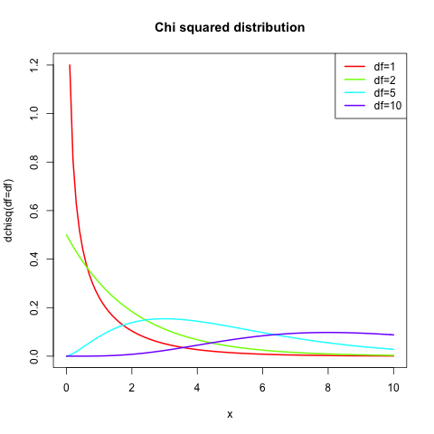
The next interesting distribution is the chi-squared (\(\chi^2\)) distribution. This distribution has also degrees of freedom (n) and it is “the distribution of a sum of squares of n independent standard normal random variables”. This might sound a little bit complicated but you will encounter tests like the Pearson \(\chi^2\)-test for which it makes perfect sense.
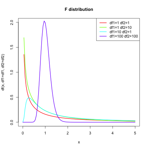
The F distribution is based on the f statistic. The f statistic is the ratio
$$\frac{\frac{s_1^2}{\sigma_1^2}}{\frac{s_2^2}{\sigma_2^2}}$$
where \(\sigma_1^2\) and \(\sigma_2^2\) are the variations of two populations and \(s_1^2\) and \(s_2^2\) are the sample variations of two samples drawn from the two populations.
In case we draw samples from the same population with variation \(\sigma_1^2 = \sigma_2^2 = \sigma^2\), the population variance cancels out and the f statistic is $$\frac{s_1^2}{s_2^2}$$.
The degrees of freedom for this distribution are based on the two samples sizes \(n_1\) and \(n_2\) and are computed as \(d_1 = n_1\) and \(d_2 = n_2\).
As soon as you have chosen a reference distribution (or you have looked it up in a statistics book ;)), you can compute the p-value. Previously people have been using tables because computing it was exhaustive. Nowadays every statistics program and even calculators can compute the p value for a given test statistic T. The first parameter \(1.96\) to each function is a made up test statistic T.
pnorm(1.96) # 0.9750021
1-pnorm(1.96) # 0.0249979
2*(1-pnorm(1.96)) # 0.04999579
The first call pnorm(1.96) returns a rather large value, which is the area under the normal distribution curve (or bell curve) in \(]-\infty; T]\), which is rather useless. What we actually want is the area in \([T; \infty[\) which is achieved by the second line and in case you need the area two-sided, just multiply it by 2 (but only because the bell curve is symmetric).
1-pt(1.96, df=1) # 0.1501714
1-pt(1.96, df=30) # 0.02967116
1-pt(1.96, df=100) # 0.02638945
For easier comparison I used \(T=1.96\) again as a sample test statistic and we can see the higher the degrees of freedom are, the closer the value gets to the p-value computed by the normal distribution. This property is what usually is known as “heavy tails”, which means that “more area” is between \(T\) and \(\infty\) in a Student’s t distribution than for a normal distribution.
1-pchisq(1.96, df=1) # 0.1615133
1-pchisq(1.96, df=5) # 0.8546517
It is obvious that here for the same T completely different p values are computed. It can also be seen that the degrees of freedom have a big influence.
1-pf(1.96, df1=1, df2=1) # 0.3948631
1-pf(1.96, df1=5, df2=5) # 0.2389522
Here the situation is similar, the p-value for the same test statistic T is very different.
4. Compare to an appropriate \(\alpha\)-value
When you choose an \(\alpha\)-value you have to think of it as the probability to reject the null hypothesis incorrectly. This is usually called the type I error, whereas the type II error is failing to reject the null hypothesis. There are many resources on type I and type II errors available online, e.g. this wikipedia page, which does a pretty good job on explaining it.
For single tests the most used \(\alpha\)-value is 5%.
When performing multiple tests, one has to consider the multiple comparisons problem. This problem, and how to deal with it (keyword multiple testing correction) I will dwell on when I write about such tests.
3. + 4. Directly compare test statistic
When you think about everything that you learned about test statistic and the p-value and \(\alpha\)-value you might see that you could directly compare the test statistic t (that was computed in step 2) to z-score, t-score, F-score or \(\chi^2\)-score (depending on your distribution). This can be done to decide whether to reject or accept the null hypothesis instead of the above presented steps 3 and 4.
Once again you can use this table, but you can also use any statistics program, but this time you do not compute the probability for a given score, but the score for a given probability, more precisely, the \(\alpha\)-value (in R this is qnorm() instead of pnorm()).
That means e.g. when you want to compare to a normal distribution with an \(\alpha\)-value of 5%, you look for the value 0.975 in the table and then you get the value 1.96.
This value 1.96, often called u, is the threshold for the rejection region:
- \( |t| \ge |u| \) : reject \(H_0\)
- \( |t| \lt |u| \) : don’t reject \(H_0\)
Conclusion
So, I hope this post gives you a good overview about the concept of statistical testing. The next two or more posts (usually my posts tend to get longer than anticipated, so I will probably have to split them up) will deal with different statistical tests for which it is necessary that you understand most of what I wrote today. Or maybe you will better understand this introduction when you see an actual test.
Source code
I put all source code for the plots and examples into one file distributions.R.