This time I am going to show you how to perform PCA and ICA. In the next one or two posts I will show you Factor Analysis and some scaling and projection methods.
The idea for this mini-series was inspired by a Machine Learning (Unsupervised) lecture I had at university.
The source code for this post can be downloaded here.
Contents
Motivation
Some data has many dimensions / features, but for classification often a small subset of dimensions would be sufficient, therefore different dimensionality reduction methods can be applied to find a meaningful subset.
Data
For showing these unsupervised techniques I use the wine dataset, consisting of 3 classes (different cultivars) and 13 features (quantities of components).
winedata=read.csv("wine.data.txt",sep=",", header=F)
wine_s<-scale(winedata[,2:14])
Principal Component Analysis (PCA)
PCA is a method to find variance in the data. It transforms the coordinate system such that the data has the highest variance along the first component, the second highest along the second component, ...
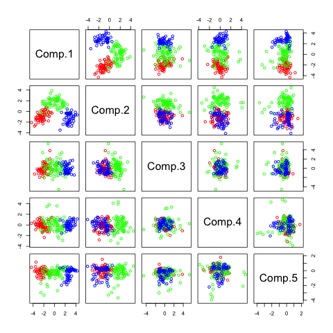
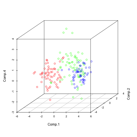
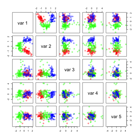
library(scatterplot3d)
pc<-princomp(wine_s)
summary(pc)

pairs(pc$scores[,1:5], col=rainbow(3)[winedata[,1]], asp=1)

scatterplot3d(pc$scores[,c(1,2,4)], color=rainbow(3)[winedata[,1]])
The output of summary is the following (showing only the first 4 components, there are 13 altogether):
Importance of components:
| Comp.1 | Comp.2 | Comp.3 | Comp.4 | |
| Standard deviation | 2.1631951 | 1.5757366 | 1.1991447 | 0.9559347 |
| Proportion of Variance | 0.3619885 | 0.1920749 | 0.1112363 | 0.0706903 |
| Cumulative Proportion | 0.3619885 | 0.5540634 | 0.6652997 | 0.7359900 |
This tells us that the first component explains 36.1 % of the variance, component 2 explains 19 % of the variance and so on...
The first graph shows the pairwise plots of the first 5 principal components (PCs). Each plot can be seen as a transformation in a 2-dimensional space where the 2 components are the new coordinate system.
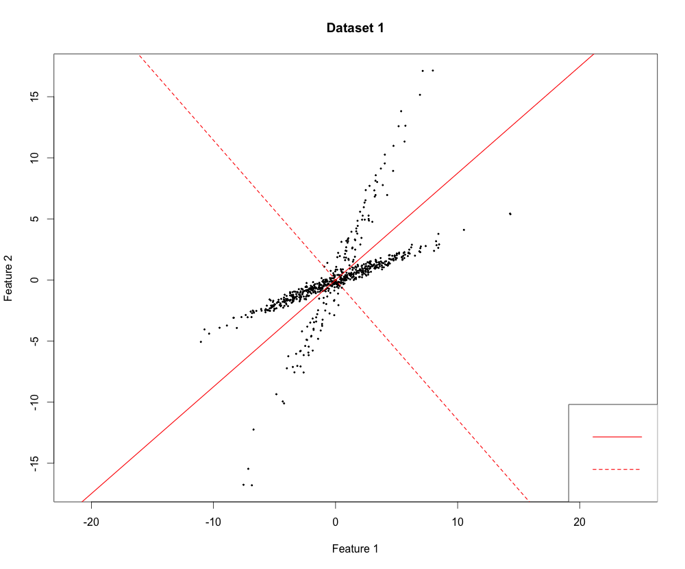
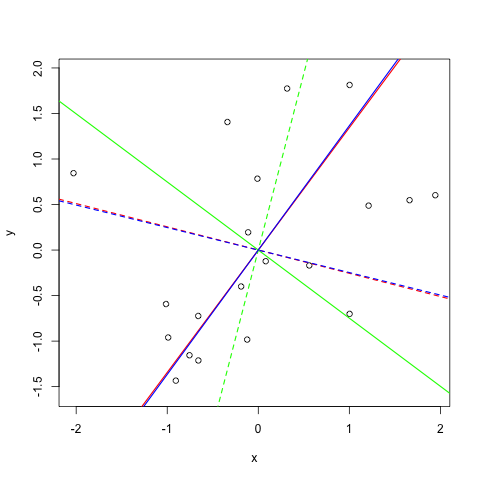
Representation of principal components on a random dataset
For better understanding I plotted the PCs I received (but on a different dataset). It is a good dataset to show how PCA works because you can clearly see that the data varies most along the first principal component. Since it is a 2-dimensional dataset, the second PC is simply the orthogonal vector to the first PC.
Independent Component Analysis (ICA)
The purpose of ICA is to find independent components in the data. In contrast to PCA you do not automatically get the same amount of components as you have dimensions. Independent components also do not have to be orthogonal and they are not ranked (there is no "most independent component").
library(fastICA)
ica<-fastICA(wine_s, n.comp=5)
ica8<-fastICA(wine_s, n.comp=8)

pairs(ica$S, col=rainbow(3)[winedata[,1]])

pairs(ica8$S, col=rainbow(3)[winedata[,1]])

plot(ica$S[,1], ica$S[,1], col=rainbow(3)[winedata[,1]], xlab="Comp 1", ylab="Comp 1")
You see that I used a parameter called n.comp which tells the method how many independent components I want. The first two plots show this:
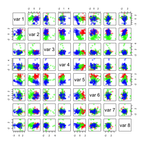
Not many of these components seem useful, in the first figure the 2 most useful components with regards to separation seem to be IC1 and IC5. In the second figure it seems to be IC1 and IC8. If you look closely you can see that these two components are the same in the 2 figures. IC1 (first fig.) and IC8 (second fig.) seems to be able to separate the data on its own.
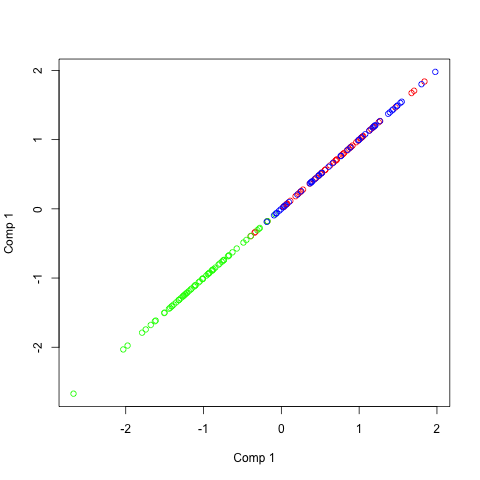
Representation of independent components on a random dataset
As you can see in the source code (link at the top of this post) I introduced some dependence between the two variables. You can see what I have mentioned before, the vectors are not orthogonal. But what you can also see is important: The angles between the two components in the same color are always the same.
Is it valid to reduce dimensionality of the data with PCA before running nonlinear dimensionality reduction?
Is PCA a good approach for reducing dimensionality in a high-dimensional multivariate time series?
Hi, I haven’t used PCA on high-dimensional multivariate time series but PLS (partial least squares) which also reduces dimensionality in a very similar way. PLS works pretty good for many applications, so I can imagine that PCA will also work but it always depends on the data! Can you provide more details?
I’m also curious as to how it compares with PLS. PLS is supervised and is prone to overfitting, so that’s one obvious difference. It’s not clear to me from this post what “independent components” are. Does that mean variables are only included in one component? (as opposed to PCA where all components include all variables, just weighted differently).
Why ICA1 & IC5 are the most important figure1 !!!!!