This time I am going to show you how to perform Factor analysis. In the next post I will show you some scaling and projection methods.
The idea for this mini-series was inspired by a Machine Learning (Unsupervised) lecture I had at university.
The source code for this post can be downloaded here.
The first part of this mini-series can be found here: [Dimensionality Reduction #1] Understanding PCA and ICA using R
Contents
Factor analysis (FA)
Factor analysis explains the variability of data using unobserved latent / hidden variables and noise. These hidden / latent variables are called factors. This is useful because sometimes correlation between observations can only be explained by factors.
Examples are:
- People who show good score on tests of verbal ability also show good results on other tests that require verbal abilities. Researchers explain this by one isolated factor, called verbal intelligence (psychology).
- Successfully used to identify dependencies between gene expression and conditions (bioinformatics).
- Measuring body weight and body height from people – will be very correlated and could be explained by one factor (made-up example)
The factor model is the following:
$$x = Uy + \epsilon$$
with the observations $$x$$
noise / error $$\epsilon$$
the factors $$y$$ and the factor loading matrix $$U$$
The following code shows factor analysis performed on the wine data set that I also used with PCA and ICA:
fa2<-factanal(wine_s, factors=2, scores="regression")
fa3<-factanal(wine_s, factors=3, scores="regression")
fa4<-factanal(wine_s, factors=4, scores="regression")
fa6<-factanal(wine_s, factors=6, scores="regression")

pairs(fa2$scores, col=rainbow(3)[winedata[,1]])

pairs(fa3$scores, col=rainbow(3)[winedata[,1]])

pairs(fa4$scores, col=rainbow(3)[winedata[,1]])

pairs(fa6$scores, col=rainbow(3)[winedata[,1]])
You can see, that similar to ICA, I have to tell the method how many factors I want to detect.
The following figures show separability with regard to the computed factors:
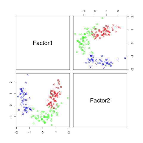
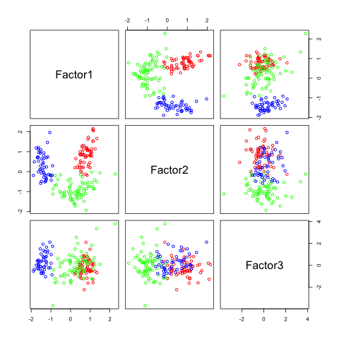
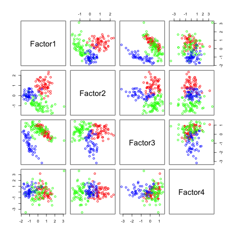
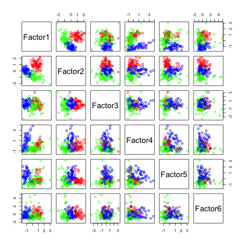
The plots with 2 and 3 factors look useful, but after that it gets very messy. This is an indicator that there not so many latent variables in the dataset.
For a better understanding I created a dataset for which we can see the dependencies.
samples<-100
category<-c(rep(1, samples/2), rep(2, samples/2))
h1<-runif(samples, 1, 5)
h2<-rnorm(samples, category, 0.3)
data<-data.frame(x1=rnorm(samples, 10+h1, 1), x2=rnorm(samples, h1^2+3*h2, 1), x3=h1+h2+rnorm(samples,0, 0.9), x4=rnorm(samples, 20*h1+h2, 2), x5=14*h1*h2+rnorm(samples, 0, 1))
png("fa_dim5.png")
plot(data, col=rainbow(4)[category])
dev.off()
First, I create a category variable, so we can color our samples and we have to groups with slightly different features. Then I create two different hidden factors h1 and h2. The first is independent from the categories but the second depends on the category value.
Then I create a data set with features that all depend on the hidden variables in some way and have some additional Gaussian noise.
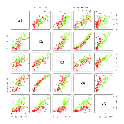
In the figure above we see the five features created. Many of them are highly correlated but they do not look to be easily separable.
For that purpose we apply factor analysis with factors=2.
fa<-factanal(data, factors=2, scores="regression")
fa$loadings
png("fa_computed.png")
pairs(fa$scores, col=rainbow(4)[category])
dev.off()
Output of fa$loadings:
Loadings:
Factor1 Factor2
x1 0.603 0.469
x2 0.614 0.786
x3 0.421 0.705
x4 0.842 0.535
x5 0.822 0.565
Factor1 Factor2
SS loadings 2.302 1.941
Proportion Var 0.460 0.388
Cumulative Var 0.460 0.849
In this output we can see how much each factor influences each feature (as computed by the factor analysis model). Interesting are the last two lines, the amount of variance explained by the factor analysis model. In PCA the last cumulative variance value would be 1. But since factor analysis does not explain all variance (the error term accounts for some of it), some variance is "lost".
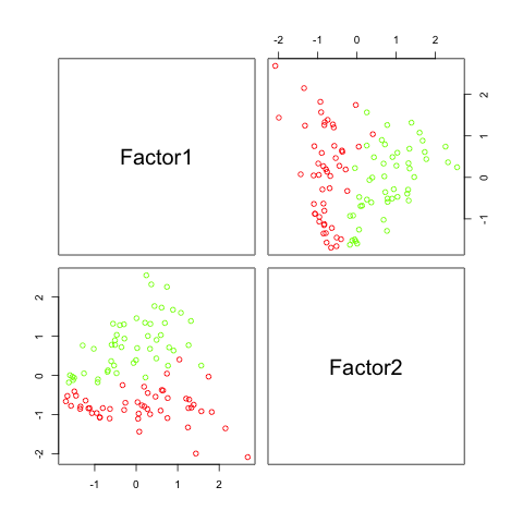
The results in the figure above look pretty promising. It can be seen that factor 2 (which corresponds to h2 by coincidence) is sufficient to separate the data. Factor 1, which corresponds to h1 does not separate the data at all, but that is because I created it independently from category.
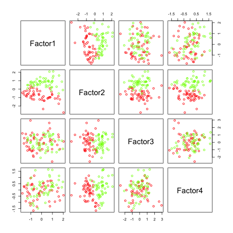
Two see, like above, what happens if we want to compute many factors, I added some features (factanal() can not compute 4 factors for only 5 features).
data1<-data.frame(x1=rnorm(samples, 10+h1, 1), x2=rnorm(samples, h1^2+3*h2, 1), x3=h1+h2+rnorm(samples,0, 0.9), x4=rnorm(samples, 20*h1+h2, 2), x5=14*h1*h2+rnorm(samples, 0, 1), x6=h1+rnorm(samples, 0, 3), x7=h1*h2*3+rnorm(samples, 0, 4), x8=6*h2+rnorm(samples, 0, 5))
plot(data1, col=rainbow(4)[category])

fa_4<-factanal(data1, factors=4, scores="regression")
fa_4$loadings
png("fa4_computed.png")
pairs(fa_4$scores, col=rainbow(4)[category])
dev.off()
Again, factor 2 seems to be most promising. All the others do not add any additional information.
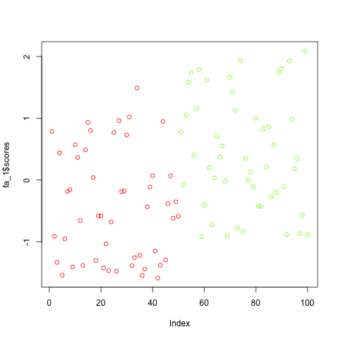
Just for demonstration purpose I also computed the factor analysis model using factors=1 which shows how easy you can reduce a dataset of 5 features to one dimension if the data is highly correlated and depends on latent factors:
Comparison of the 3 methods
Here I do not give a comparison of the results (because I promised it for the next post), but a short summary of the properties:
| PCA | ICA | FA | |
| geometrical abstractions | - | causes of the data | |
| explain all variance | - | explain common variance | |
| first l with max. variance | - | variance shared | |
| no noise | no noise | additive noise (variance lost) | |
| components are ranked | no ranking | no ranking |
Sources
Most of the knowledge I have about this topic is from machine learning and data analysis courses at university, I can only recommend the Basic Methods of Data Analysis Lecture.
A post well done – nicely summarizing features of the different transformations in comparison to each other. If more people would understand these methods in detail, they would probably be used more appropriately on some data out there 😉
Wish you success on your future posts and projects!